Case study: mtDNA haplogroups and HIV status in Botswana

Work a real dataset end-to-end: from a sequencing-derived haplogroup call to a hypothesis test — and to the reason the hypothesis test cannot be trusted.

Why this module

Every dataset you have analysed so far in this series was chosen because it behaves. This one does not. It is a real study: 338 participants from Botswana, mitochondrial genomes sequenced, haplogroups assigned with HaploGrep 3, and paired with HIV status.

The scientific question was simple: does mitochondrial ancestry associate with HIV status?

The answer turns out to be “we cannot tell from this data” — and finding out why is the actual lesson. Learning to recognise that situation is worth more than another clean p-value.

Learning objectives

By the end of this module you should be able to:

Load and inspect a real haplogroup dataset with the tidyverse.
Derive a coarser grouping (macro-haplogroup) from a fine-grained label.
Build and interpret a contingency table.
Choose between a chi-squared and a Fisher exact test, and know why.
Detect confounding before you believe a result.

The data

This is a synthetic teaching dataset

The real Botswana cohort is not distributed with this workshop — it carries participant HIV status and stays private. The block below regenerates a synthetic dataset with the same shape (338 participants, L-lineage haplogroups) and, crucially, the same fatal design flaw: sex perfectly confounded with HIV status. Every number on this page comes from that synthetic data. Do not cite any of it as a real epidemiological result.

set.seed(1)
n <- 338

# Macro-haplogroups: L0 dominant, L1 rare — as in the real Southern African cohort
macro <- sample(c("L0", "L1", "L2", "L3"), n, replace = TRUE,
                prob = c(0.53, 0.05, 0.16, 0.24))

# Fine-grained labels, long-tailed so most have only a handful of carriers
sub_pool <- c("a1","a1b","a1b1","a2","a2a","a2a1","a2a2","a2a2a","b1","b2",
              "b2a","b2b","c","c1","d","d1","d1a","d1b","d1b1","d1b2",
              "d1b2b","d1b2b1","d1b2b1b","d3","d3a","d3b","e","e1","e1a",
              "e1a1","e1a1a","f","f1","f1a","f1b","f1b1","g1","h","h1","k1a")
haplogroup <- paste0(macro,
  sample(sub_pool, n, replace = TRUE, prob = rev(seq_along(sub_pool))^1.3))

# The sampling artifact: every man entered through the HIV-negative arm, so the
# HIV-positive group is women only. HIV status is otherwise independent of
# haplogroup — there is no real haplogroup effect built in.
sex <- sample(c("F", "M"), n, replace = TRUE, prob = c(0.88, 0.12))
hiv_status <- ifelse(sex == "M", "negative",
                     sample(c("positive", "negative"), n,
                            replace = TRUE, prob = c(0.75, 0.25)))

mtdna <- tibble(
  participant_id   = sprintf("BW_%04d", sample(n)),
  haplogroup       = haplogroup,
  macro_haplogroup = macro,
  sex              = sex,
  hiv_status       = hiv_status
)
glimpse(mtdna)

Rows: 338
Columns: 5
$ participant_id   <chr> "BW_0331", "BW_0084", "BW_0329", "BW_0175", "BW_0013"…
$ haplogroup       <chr> "L0c", "L0f", "L3f1b", "L2a2", "L0b2b", "L2a2a2a", "L…
$ macro_haplogroup <chr> "L0", "L0", "L3", "L2", "L0", "L2", "L2", "L3", "L3",…
$ sex              <chr> "F", "F", "F", "F", "F", "F", "F", "F", "F", "F", "F"…
$ hiv_status       <chr> "positive", "negative", "negative", "positive", "posi…

Five columns:

Column	Meaning
`participant_id`	De-identified participant code
`haplogroup`	Full HaploGrep 3 call, e.g. `L0d1b2b1b`
`macro_haplogroup`	First two characters, e.g. `L0`
`sex`	Recorded sex
`hiv_status`	`positive` / `negative`

Where macro_haplogroup comes from

Haplogroup labels are hierarchical: L0d1b2b1b sits inside L0d1b2, inside L0d, inside L0. Truncating to two characters collapses the 97 fine-grained labels here into 4 macro-groups. We do this because most of those labels have only a handful of participants — far too few to test.

Step 1 — Look before you test

mtdna |> count(macro_haplogroup, sort = TRUE)

# A tibble: 4 × 2
  macro_haplogroup     n
  <chr>            <int>
1 L0                 197
2 L3                  78
3 L2                  48
4 L1                  15

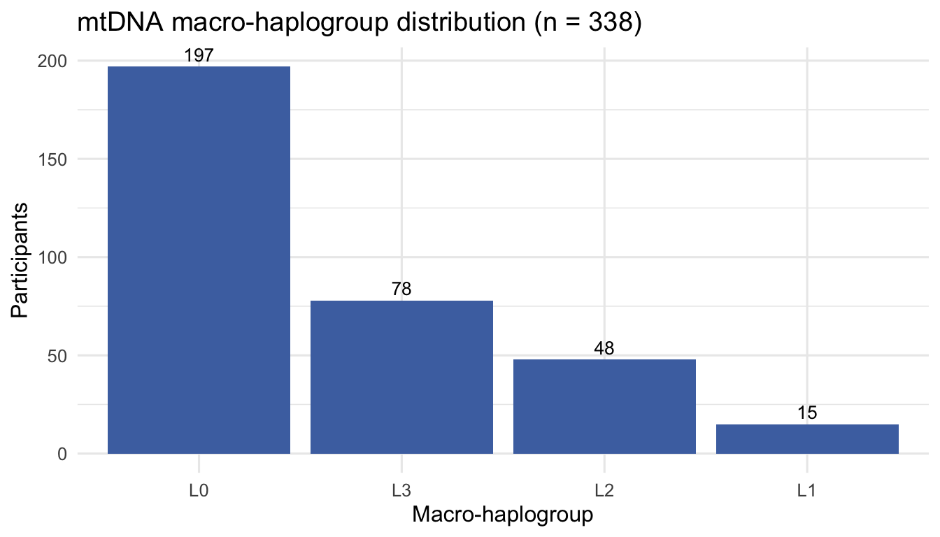
Four macro-haplogroups, all within the L lineage — as expected for a Southern African cohort. L0 dominates, which is consistent with L0 being the deepest branch of the human mtDNA tree and common in Khoe-San-related ancestry.

mtdna |>
  count(macro_haplogroup) |>
  ggplot(aes(x = fct_reorder(macro_haplogroup, -n), y = n)) +
  geom_col(fill = "#4C72B0") +
  geom_text(aes(label = n), vjust = -0.4, size = 3.5) +
  labs(x = "Macro-haplogroup", y = "Participants",
       title = "mtDNA macro-haplogroup distribution (n = 338)") +
  theme_minimal(base_size = 12)

Step 2 — The contingency table

tab <- table(mtdna$macro_haplogroup, mtdna$hiv_status)
tab

    
     negative positive
  L0       71      126
  L1        4       11
  L2       15       33
  L3       31       47

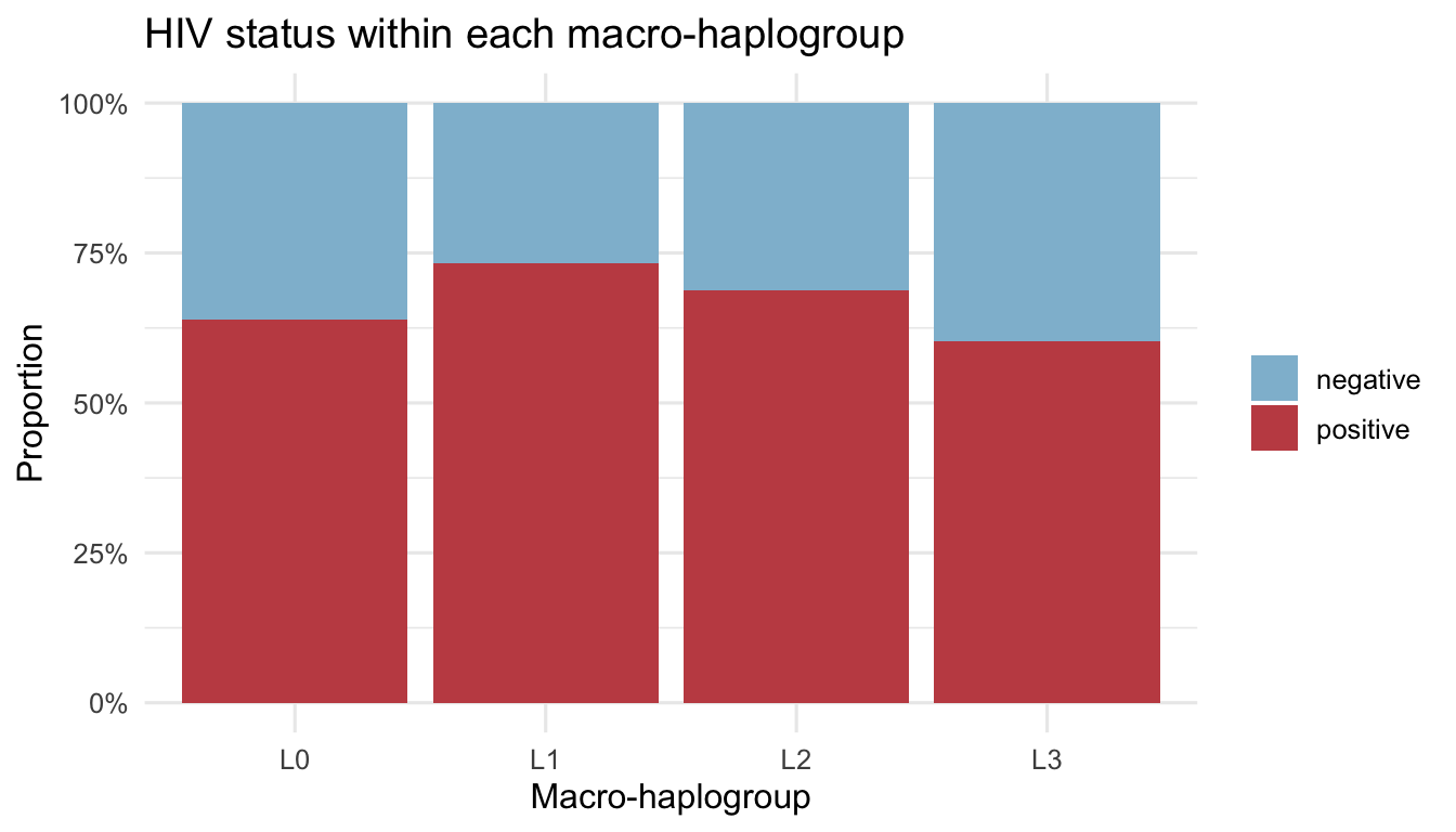
Eyeball it before testing. Roughly two-thirds of every row is positive. The rows look similar — which is already a hint about what the test will say.

mtdna |>
  ggplot(aes(x = macro_haplogroup, fill = hiv_status)) +
  geom_bar(position = "fill") +
  scale_y_continuous(labels = scales::percent) +
  scale_fill_manual(values = c(negative = "#8FBCD4", positive = "#C44E52")) +
  labs(x = "Macro-haplogroup", y = "Proportion", fill = NULL,
       title = "HIV status within each macro-haplogroup") +
  theme_minimal(base_size = 12)

Step 3 — Test it

chisq.test(tab)


    Pearson's Chi-squared test

data:  tab
X-squared = 1.5096, df = 3, p-value = 0.6801

The p-value is well above 0.05 — no evidence of association.

chi-squared or Fisher?

Chi-squared is an approximation that degrades when expected cell counts fall below ~5. Check first:

chisq.test(tab)$expected |> round(1)

    
     negative positive
  L0     70.5    126.5
  L1      5.4      9.6
  L2     17.2     30.8
  L3     27.9     50.1

The L1 row is thin. Fisher’s exact test does not rely on the approximation:

fisher.test(tab, simulate.p.value = TRUE, B = 10000)


    Fisher's Exact Test for Count Data with simulated p-value (based on
    10000 replicates)

data:  tab
p-value = 0.6984
alternative hypothesis: two.sided

Both agree — no association. When two tests with different assumptions agree, you can stop worrying about which one to report.

Step 4 — The part that matters

Before you write “no association between mtDNA haplogroup and HIV status” in a manuscript, run one more line:

table(mtdna$sex, mtdna$hiv_status)

   
    negative positive
  F       76      217
  M       45        0

Read that table carefully.

Every single male in this cohort is HIV-negative. Every HIV-positive participant is female.

That is not biology. No cohort in Botswana looks like this by chance — HIV prevalence in men is not zero. This is a sampling artifact: the HIV-negative comparison group was recruited in a way that pulled in the only men in the study.

The consequence is severe. Sex is perfectly confounded with HIV status, so:

Any haplogroup–HIV signal is inseparable from a haplogroup–sex signal.
You cannot adjust for sex. Adjustment needs some overlap — HIV-positive men or HIV-negative-only women to compare against. There are none.
The null result above is therefore uninformative, not reassuring. We did not find “no effect”; we found that this design cannot measure the effect.

The transferable lesson

A p-value answers the question you asked. It cannot tell you the question was unanswerable. Always cross-tabulate your exposure against your key covariates before you interpret a test. One table() call would have saved this analysis.

Because mtDNA is maternally inherited, a sex imbalance is especially dangerous here — but this failure mode is completely general.

Exercises

1. Restrict the analysis to women only and re-run the test. What is the p-value now? Does restricting fix the confounding, and what did you pay for it?

women <- mtdna |> filter(sex == "F")
# your code here

2. Collapse to L0 vs everything else and test with fisher.test(). Does a binary comparison change the conclusion?

3. The fine-grained haplogroups were collapsed to 4 macro-groups. Count participants per full haplogroup. How many have fewer than 5? What would happen to a chi-squared test run on the uncollapsed table?

4. Discussion. You are handed this dataset and asked to publish the null result. What do you tell the team, and what would you need to collect to answer the original question properly?

What to take away

Real data arrives with defects that no amount of correct statistics repairs.
Look at marginals and cross-tabs before testing.
A null result from a confounded design is not a null result.
Reporting why a question cannot be answered is a legitimate scientific contribution.

About this dataset

Synthetic. It is generated in the code block above to mirror a real study of mitochondrial genomes in Botswana — the same size, the same L-lineage haplogroup structure, and the same sex/HIV confounding that makes the real analysis uninterpretable — without using any real participant data. The real cohort is not distributed: it carries HIV status and remains private. Nothing on this page should be read as an actual result from the Botswana study.